Assessing Data Normality: How to Do It Correctly
Assessing the normality of data distributions is one of the first stages of statistical analysis in…
Read more >Assessing the normality of data distributions is one of the first stages of statistical analysis in medical research. In many publications, however, the entire procedure is described in a single sentence: “Normality was assessed using the Shapiro–Wilk test.” Depending on the resulting p-value, the authors then automatically choose either a parametric or a non-parametric test.
Although straightforward, this approach is not always appropriate. Normality assessment should not be based solely on the result of a single statistical test. It should also take into account histograms, Q–Q plots, skewness, kurtosis, outliers, sample size and the assumptions of the statistical method that is being considered.
The Shapiro–Wilk test is a useful diagnostic tool, but it should not be treated as an automatic switch between Student’s t-test and the Mann–Whitney U test.
In medical statistics, the most important question is not: “Are the data perfectly normally distributed?” Instead, we should ask: “Could the characteristics of the data adversely affect the statistical method we intend to use?”
A variable is said to follow a normal distribution, also known as a Gaussian distribution, when most observations are concentrated around the average value and very low or very high values occur less frequently. When presented graphically, such a distribution resembles a symmetrical bell-shaped curve.
In a perfectly normal distribution, the observations are symmetrically distributed on both sides of the centre. The mean, median and mode are equal. Most observations are located close to the mean: approximately 68% fall within one standard deviation of the mean, while approximately 95% fall within two standard deviations.
In real-world medical data, a perfect bell-shaped distribution is uncommon. Minor deviations from this shape occur frequently and do not necessarily create a problem for subsequent statistical analysis.
Assessing the distribution of the data helps determine whether the selected descriptive measures and planned statistical analyses are appropriate for the actual structure of the dataset.
In medical statistics, this is particularly important when choosing between:
Normality assessment may also help determine whether the assumptions of a planned statistical test or model are satisfied, whether the result may be disproportionately influenced by individual extreme observations and whether a data transformation should be considered.
The objective is therefore not simply to classify a distribution as “normal” or “non-normal”. The real purpose is to establish whether the characteristics of the data could undermine the reliability of the planned statistical analysis.
A non-normal distribution should not automatically be interpreted as an indication that a non-parametric test is required. A more important consideration is whether the type and magnitude of the deviation could materially affect the performance of the selected statistical method.
Good statistical practice involves combining several diagnostic methods rather than mechanically interpreting a single p-value.
A practical assessment of medical data should include the following steps:
Normality should therefore be treated as a diagnostic issue rather than as a single formal test that produces a simple “yes” or “no” decision.
Before assessing normality, researchers must ensure that the dataset itself is correct. A single data-entry error may substantially alter the appearance of a histogram, the result of a normality test and the conclusions drawn from the analysis.
A simple example is a recorded value of 450 instead of 45. Such an error may be responsible for the apparent asymmetry of the entire distribution. Similarly, a recorded BMI of 285 is more likely to represent 28.5 than a genuine clinical observation.
The dataset should therefore be checked for:
A histogram is a simple bar chart showing how many observations fall within consecutive ranges of values. It allows researchers to quickly identify whether the data are approximately symmetrical, skewed or multimodal, meaning that the distribution has more than one prominent peak.
A histogram can also help identify extreme observations.
An example of a BMI histogram is presented below.
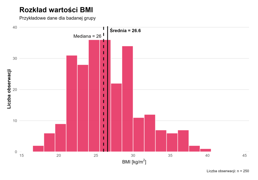
In practice, a histogram provides an initial assessment of:
Although histograms are extremely useful, they have an important limitation: their appearance depends on the number and width of the selected intervals, commonly referred to as bins.
The same dataset may look different after changing the histogram settings. Bins that are too wide may conceal irregularities, whereas bins that are too narrow may overemphasise random fluctuations.
The histogram below presents the same BMI dataset as the previous figure, but with a different number and width of bins.
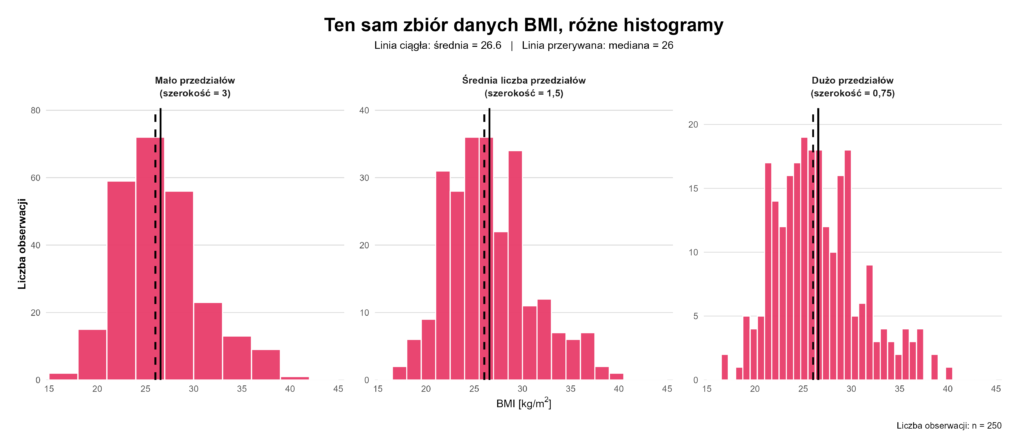
Histograms may also be unstable and difficult to interpret in small samples. With only 10 or 15 observations, researchers should not expect to see a perfectly smooth bell-shaped curve, even when the observations genuinely come from a normally distributed population.
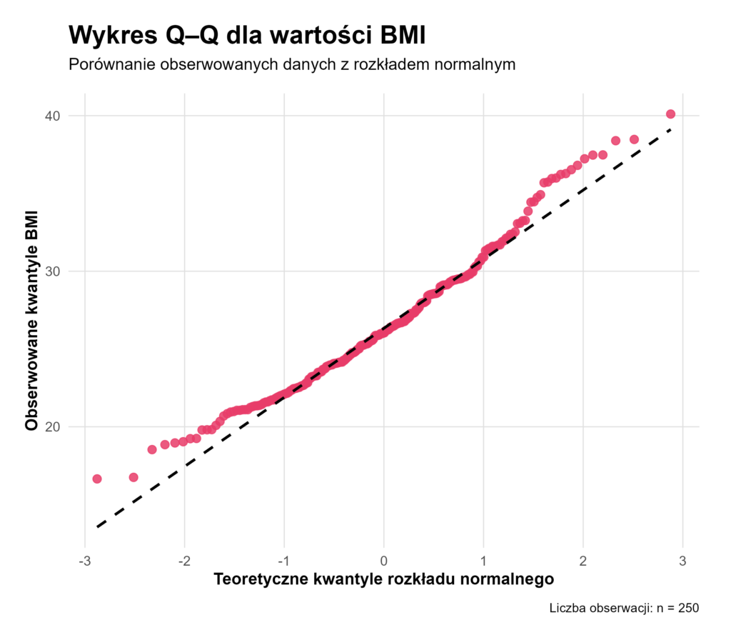
A Q–Q plot, or quantile–quantile plot, compares the observed data with the values expected under a normal distribution.
In simplified terms, when the plotted points follow an approximately diagonal straight line, the distribution may be considered reasonably close to normal.
Characteristic deviations from the reference line may indicate:
A single deviation at the edge of a Q–Q plot does not necessarily justify rejecting parametric methods. Its relevance depends on the magnitude of the deviation, the sample size and whether the unusual observation represents a data error or a valid clinical result.
Skewness is a descriptive statistic that indicates whether a distribution is symmetrical or whether it has a longer tail on one side.
Positive, or right, skewness means that most observations are concentrated at lower values, while a small number of high observations extend the right tail of the distribution. Negative, or left, skewness describes the opposite pattern.
Right-skewed distributions are very common in medical data. Examples include:
In such cases, most patients have low or moderate values, while a small group or individual patients have very high values.
Kurtosis describes certain aspects of the shape of a distribution, particularly the concentration of observations and the behaviour of its tails. High kurtosis may indicate heavy tails and an increased probability of extreme observations.
There are no universal skewness or kurtosis thresholds that can definitively determine whether a parametric analysis is acceptable in every study.
Frequently cited thresholds, such as ±1 or ±2, should be treated as general guidelines rather than absolute decision criteria.
The Shapiro–Wilk test evaluates the null hypothesis that the observed data come from a normally distributed population.
It is a useful statistical test, but its result must be interpreted carefully.
The main principles of interpretation are as follows:
Consequently, as the sample size increases, it becomes progressively less reasonable to select a statistical method solely on the basis of the Shapiro–Wilk p-value.
This issue is discussed in more detail in the article: Sample Size and Data Normality: Can the Shapiro–Wilk Test Be Misleading?
This is one of the most common misunderstandings in medical data analysis. The answer is: not always. It depends on the statistical method being used.
For example, in a paired Student’s t-test, the analysis concerns the differences between two paired measurements. It is therefore the distribution of these differences—not the separate distributions of the “before” and “after” measurements—that should be assessed for normality.
In linear regression, the normality assumption primarily concerns the random error component, which is usually evaluated by analysing the model residuals. The independent variables themselves are not required to follow a normal distribution.
Moreover, not all statistical methods require normality assessment.
Logistic regression is one example. Its dependent variable is usually binary and therefore, by definition, cannot follow a normal distribution.
Before performing the Shapiro–Wilk test, researchers should first establish which variable or component of the model is actually expected to follow a normal distribution and therefore requires assessment.
No. A Shapiro–Wilk result of p < 0.05 indicates that a deviation from a perfectly normal distribution has been detected. However, it does not explain:
The result also does not indicate whether a non-parametric method answers the same research question.
The Mann–Whitney U test is not a simple non-parametric substitute for Student’s t-test. Student’s t-test evaluates differences between means, whereas the Mann–Whitney U test compares distributions or ranks.
Interpreting the Mann–Whitney U test as a test of differences between medians requires additional assumptions, including distributions of a similar shape in the compared groups.
The choice of statistical test should therefore be based on:
It should not be determined solely by whether the Shapiro–Wilk p-value falls above or below 0.05.
The statement “Normality was assessed using the Shapiro–Wilk test” is technically correct but usually incomplete.
It does not indicate whether the authors examined diagnostic plots, evaluated outliers, considered skewness or took the sample size into account.
A more informative description could be:
The distributions of continuous variables were evaluated using histograms and Q–Q plots, together with skewness and kurtosis statistics. The Shapiro–Wilk test was used as a supplementary formal method for assessing deviations from normality. Group sizes, the presence of outliers and the robustness of the planned statistical tests to violations of the normality assumption were also considered when selecting the statistical methods.
For linear regression, it is useful to specify that the residuals of the model were evaluated rather than all variables separately.
For example: The normality assumption was evaluated by examining the distribution of the model residuals and the Q–Q plot of the residuals.
One of the most common errors is treating p ≥ 0.05 in the Shapiro–Wilk test as proof that a distribution is normal.
Other frequent problems include:
Although this procedure may appear objective, it does not adequately account for the properties of the statistical methods, the sample size, the research objective or the clinical relevance of the observed deviations.
Professional statistical analysis of medical data involves understanding the structure of the dataset and selecting a method that answers the appropriate research question while providing reliable results.
When preparing a statistical analysis for a scientific paper, publication or doctoral dissertation, it is advisable to plan the assessment of data distributions before conducting the main analyses. This facilitates the selection of appropriate statistical methods, improves the reporting of results and helps researchers respond to potential comments from reviewers.
Need support with your research? Learn more about our professional medical statistics services and discover how we can help you plan, analyse and report your study.